28  모델 해석

Keywords

python, 전처리, 통계, 가설검정, 기계학습, 회귀, 분류, 군집, 모델 학습, 모델 평가

모델 해석(Model Interpretation)은 머신러닝 모델이 어떻게 예측하는지 이해하고 설명하는 과정이다. 모델이 복잡해질수록 블랙박스처럼 작동하지만, 실무에서는 “어떤 변수가 중요한가?”, “왜 이런 예측이 나왔는가?”, “모델이 편향되지 않았는가?”를 반드시 답해야 한다. 모델 해석은 선택이 아닌 필수이며, 신뢰성 있는 의사결정을 위해 반드시 필요하다. 이 장에서는 특성 중요도, Permutation Importance, SHAP, PDP 등 주요 모델 해석 기법을 학습한다.

예제: 데이터 로드

import seaborn as sns
import pandas as pd
import numpy as np
import matplotlib.pyplot as plt
from sklearn.model_selection import train_test_split
from sklearn.ensemble import RandomForestClassifier

# 데이터 로드
df = sns.load_dataset("penguins").dropna()

# 특성과 타겟 준비
X = df[["bill_length_mm", "bill_depth_mm", "flipper_length_mm", "body_mass_g"]]
y = df["species"]

# 데이터 분할
X_train, X_test, y_train, y_test = train_test_split(
    X, y, test_size=0.2, random_state=42, stratify=y
)

print("데이터 크기:", X.shape)
print("특성:", X.columns.tolist())
print("타겟:", y.name)

데이터 크기: (333, 4)
특성: ['bill_length_mm', 'bill_depth_mm', 'flipper_length_mm', 'body_mass_g']
타겟: species

28.1 모델 해석의 필요성

모델 해석은 단순한 학술적 관심이 아니라 실무적 필수 요소이다.

모델 해석이 필요한 이유

이유	설명	예시
신뢰성 확보	모델 결정 근거 제시	의료 진단, 대출 심사
편향 탐지	불공정한 예측 발견	성별/인종 차별 방지
디버깅	모델 오류 원인 파악	잘못된 변수 사용 발견
규제 준수	설명 가능성 요구 충족	GDPR, 금융 규제
도메인 지식 결합	전문가 검증 가능	의학적 타당성 확인
개선 방향	모델 성능 향상 힌트	중요 변수 추가 수집

해석 가능성 vs 성능

모델	해석 가능성	성능	사용 상황
선형 회귀	매우 높음	낮음	규제 산업, 보고서
결정 트리	높음	중간	비즈니스 룰
랜덤 포레스트	중간	높음	일반적 상황
XGBoost	낮음	매우 높음	경진대회
딥러닝	매우 낮음	매우 높음	이미지, 텍스트

28.2 모델 해석의 범주

모델 해석은 전역적 해석과 국소적 해석으로 나뉜다.

전역 해석 vs 국소 해석

구분	전역 해석 (Global)	국소 해석 (Local)
질문	모델이 전반적으로 무엇을 중요하게 보는가?	이 특정 예측은 왜 이렇게 나왔는가?
대상	전체 데이터셋	개별 샘플
방법	Feature Importance, PDP	SHAP Force Plot, LIME
용도	모델 이해, 변수 선택	개별 결정 설명

28.3 특성 중요도 (Feature Importance)

특성 중요도는 모델이 예측에 각 변수를 얼마나 활용했는지 수치로 표현한 것이다.

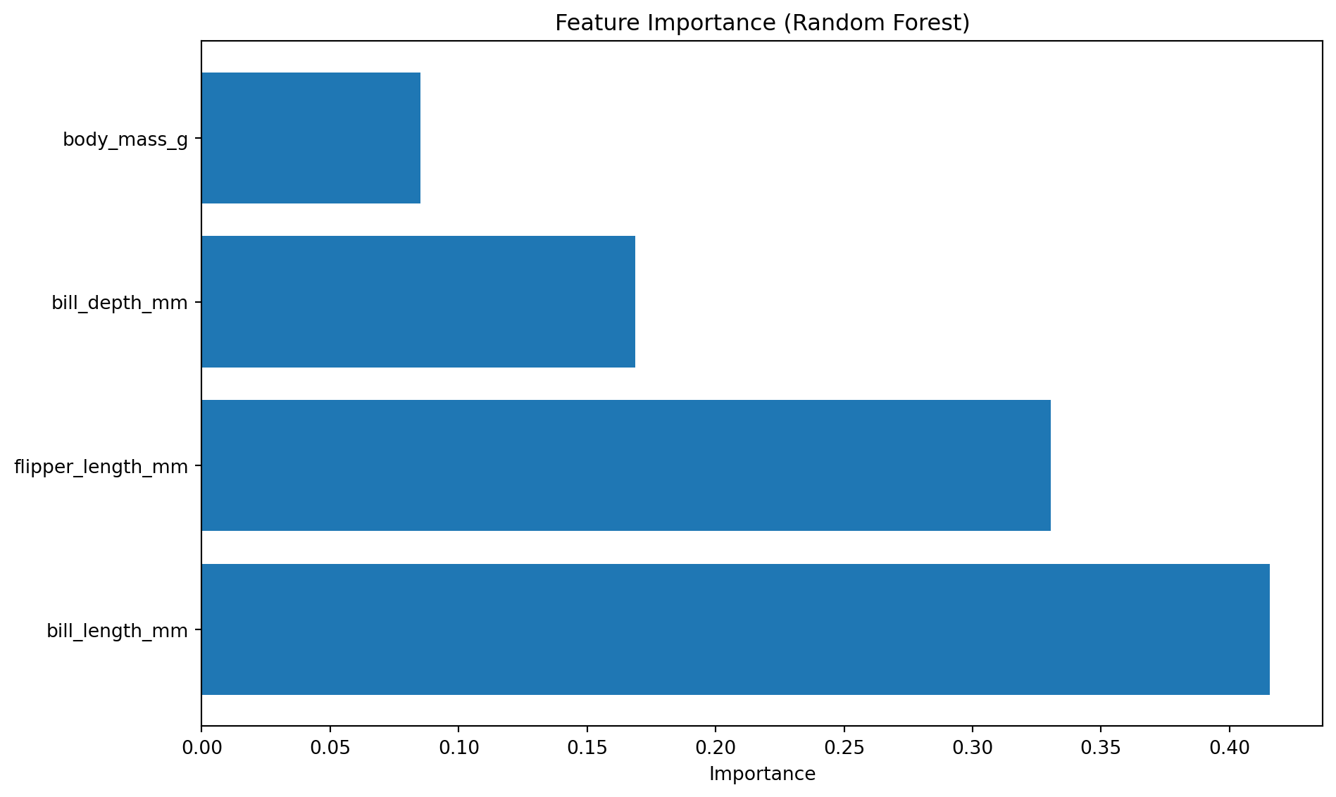
28.3.1 트리 기반 모델의 특성 중요도

트리 기반 모델(Decision Tree, Random Forest, XGBoost)은 내장 중요도를 제공한다.

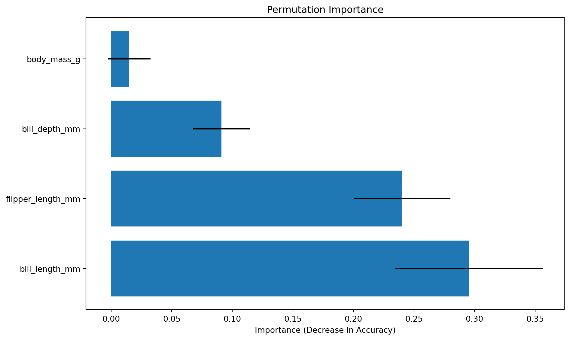
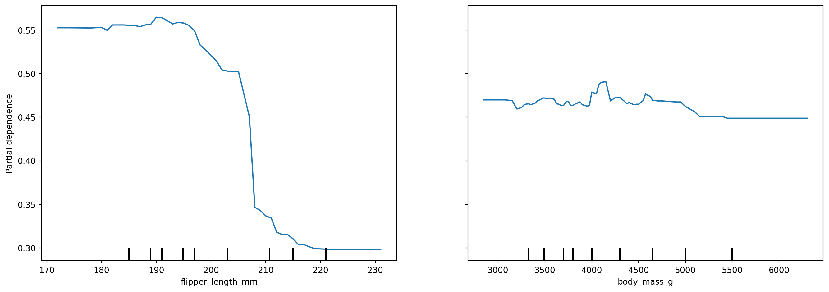
예제: 모델 학습 및 특성 중요도

# RandomForest 학습
rf = RandomForestClassifier(n_estimators=200, random_state=42)
rf.fit(X_train, y_train)

# 특성 중요도
feature_importance = pd.DataFrame({
    'Feature': X.columns,
    'Importance': rf.feature_importances_
}).sort_values('Importance', ascending=False)

print("=== RandomForest 특성 중요도 ===")
print(feature_importance)

# 시각화
plt.figure(figsize=(10, 6))
plt.barh(feature_importance['Feature'], feature_importance['Importance'])
plt.xlabel('Importance')
plt.title('Feature Importance (Random Forest)')
plt.tight_layout()
plt.show()

=== RandomForest 특성 중요도 ===
             Feature  Importance
0     bill_length_mm    0.415594
2  flipper_length_mm    0.330553
1      bill_depth_mm    0.168720
3        body_mass_g    0.085133

특성 중요도 계산 원리

• 불순도 감소: 각 특성이 분기 시 불순도를 얼마나 감소시켰는가
• 가중 평균: 모든 트리에서의 기여도 평균
• 정규화: 합이 1이 되도록 조정

해석 시 주의사항

주의점	설명
인과관계 아님	상관관계일 뿐, 인과관계 아님
상관변수 왜곡	상관성 높은 변수들 사이에서 중요도 분산
편향 가능	카디널리티 높은 변수 선호
학습 데이터 의존	테스트 성능과 무관

28.4 Permutation Importance

Permutation Importance는 특정 변수를 무작위로 섞었을 때 모델 성능이 얼마나 감소하는지로 중요도를 측정한다.

Permutation Importance 장점

• 모델 종류 무관 (모든 모델에 적용 가능)
• 실제 성능 기반 (과적합 변수 탐지)
• 상관변수 영향 적음

작동 원리

1. 기준 성능 측정 (원본 데이터)
2. 특성 하나를 무작위로 섞기
3. 성능 재측정
4. 성능 감소량 = 중요도
5. 여러 번 반복하여 평균

28.4.1 Permutation Importance 실습

예제: Permutation Importance 계산

from sklearn.inspection import permutation_importance

# Permutation Importance (테스트 데이터 기준)
result = permutation_importance(
    rf, X_test, y_test,
    n_repeats=10,
    random_state=42,
    n_jobs=-1
)

# 결과 정리
perm_importance = pd.DataFrame({
    'Feature': X.columns,
    'Importance': result.importances_mean,
    'Std': result.importances_std
}).sort_values('Importance', ascending=False)

print("\n=== Permutation Importance ===")
print(perm_importance)

# 시각화
plt.figure(figsize=(10, 6))
plt.barh(perm_importance['Feature'], perm_importance['Importance'], 
         xerr=perm_importance['Std'])
plt.xlabel('Importance (Decrease in Accuracy)')
plt.title('Permutation Importance')
plt.tight_layout()
plt.show()

=== Permutation Importance ===
             Feature  Importance       Std
0     bill_length_mm    0.295522  0.060737
2  flipper_length_mm    0.240299  0.039742
1      bill_depth_mm    0.091045  0.023552
3        body_mass_g    0.014925  0.017660

예제: Feature Importance vs Permutation Importance 비교

# 두 방법 비교
comparison = pd.DataFrame({
    'Feature': X.columns,
    'Built-in': rf.feature_importances_,
    'Permutation': result.importances_mean
})

# 순위 비교
comparison['Built-in Rank'] = comparison['Built-in'].rank(ascending=False)
comparison['Permutation Rank'] = comparison['Permutation'].rank(ascending=False)

print("\n=== 중요도 비교 ===")
print(comparison.sort_values('Permutation', ascending=False))

# 시각화
fig, axes = plt.subplots(1, 2, figsize=(14, 5))

axes[0].barh(comparison['Feature'], comparison['Built-in'])
axes[0].set_xlabel('Importance')
axes[0].set_title('Built-in Feature Importance')

axes[1].barh(comparison['Feature'], comparison['Permutation'])
axes[1].set_xlabel('Importance')
axes[1].set_title('Permutation Importance')

plt.tight_layout()
plt.show()

=== 중요도 비교 ===
             Feature  Built-in  Permutation  Built-in Rank  Permutation Rank
0     bill_length_mm  0.415594     0.295522            1.0               1.0
2  flipper_length_mm  0.330553     0.240299            2.0               2.0
1      bill_depth_mm  0.168720     0.091045            3.0               3.0
3        body_mass_g  0.085133     0.014925            4.0               4.0

28.5 Partial Dependence Plot (PDP)

PDP는 특정 변수가 변할 때 예측값이 평균적으로 어떻게 변하는지 시각화한다.

PDP의 특징

• 변수의 영향 방향(+/−) 확인
• 전역적 경향 파악
• 비선형 관계 시각화
• 다른 변수는 고정

28.5.1 PDP 실습

예제: Partial Dependence Plot

from sklearn.inspection import PartialDependenceDisplay

# PDP 생성
features = ['flipper_length_mm', 'body_mass_g']
fig, ax = plt.subplots(figsize=(14, 5))

PartialDependenceDisplay.from_estimator(
    rf, X_train, features,
    target='Adelie',
    ax=ax,
    n_jobs=-1
)
plt.tight_layout()
plt.show()

예제: 2D PDP (변수 간 상호작용)

# 2D PDP로 상호작용 확인
fig, ax = plt.subplots(figsize=(10, 8))

PartialDependenceDisplay.from_estimator(
    rf, X_train,
    features=[(0, 2)],  # bill_length_mm와 flipper_length_mm
    target='Adelie',
    ax=ax,
    n_jobs=-1
)
plt.tight_layout()
plt.show()

PDP 해석

• 상승 패턴: 변수 증가 → 예측값 증가
• 하강 패턴: 변수 증가 → 예측값 감소
• 평탄: 변수가 예측에 거의 영향 없음
• 비선형: 특정 구간에서만 영향

28.6 SHAP (SHapley Additive exPlanations)

SHAP는 게임 이론의 Shapley Value를 기반으로 각 특성의 기여도를 계산하는 현재 가장 표준적인 모델 해석 방법이다.

SHAP의 특징

특징	설명
이론적 보장	공정한 기여도 계산 (Shapley Value)
전역 + 국소	모델 전체와 개별 예측 모두 설명
방향성	양수(증가)/음수(감소) 기여도
일관성	모든 예측의 합 = 최종 예측
모델 독립적	다양한 모델에 적용 가능

SHAP 값의 핵심 개념

최종 예측 = 기준값(base value) + Σ(각 특성의 SHAP 값)

28.6.1 SHAP 실습 (Python 3.6-3.10)

SHAP는 Python 3.6~3.10에서 지원된다. Python 3.11+ 환경에서는 Permutation Importance + PDP 조합을 사용한다.

예제: SHAP 기본 사용 (Python 3.6-3.10)

# SHAP 설치 필요: pip install shap
try:
    import shap
    
    # TreeExplainer (트리 기반 모델용)
    explainer = shap.TreeExplainer(rf)
    shap_values = explainer.shap_values(X_test)
    
    # Summary Plot (전역 해석)
    print("=== SHAP Summary Plot ===")
    shap.summary_plot(shap_values, X_test, plot_type="bar")
    
    # 상세 Summary Plot (분포 포함)
    shap.summary_plot(shap_values, X_test)
    
    # Force Plot (개별 예측 해석)
    sample_idx = 0
    shap.force_plot(
        explainer.expected_value[0],
        shap_values[0][sample_idx],
        X_test.iloc[sample_idx]
    )
    
except ImportError:
    print("SHAP이 설치되지 않았거나 Python 버전이 호환되지 않습니다.")
    print("대신 Permutation Importance + PDP를 사용하세요.")

SHAP Summary Plot 해석

• 막대형 (bar): 전체 모델에서 중요한 변수 순위
• 분포형 (beeswarm):
  • 색상: 특성 값 크기 (빨강=높음, 파랑=낮음)
  • X축: SHAP 값 (양수=증가 기여, 음수=감소 기여)
  • Y축: 특성

28.7 모델 해석 방법 종합 비교

해석 방법 비교

방법	전역/국소	방향성	모델 독립	계산 비용	장점	단점
Feature Importance	전역	✗	트리만	낮음	빠름	편향 가능
Permutation Importance	전역	✗	✓	중간	신뢰	느림
PDP	전역	✓	✓	중간	직관적	상호작용 미반영
SHAP	전역+국소	✓	✓	높음	이론적 보장	매우 느림

상황별 권장 방법

상황	권장 방법	이유
빠른 탐색	Feature Importance	즉시 확인 가능
신뢰할 수 있는 전역 해석	Permutation Importance	실제 성능 기반
영향 방향 확인	PDP	비선형 관계 파악
개별 예측 설명	SHAP	완전한 설명
보고서/프레젠테이션	PDP + SHAP	시각적으로 명확

28.8 실무 활용 예제

예제: 종합 해석 리포트

# 1. Permutation Importance로 중요 변수 파악
print("=== 1. 중요 변수 파악 (Permutation Importance) ===")
print(perm_importance.head(3))

# 2. PDP로 상위 2개 변수 영향 확인
print("\n=== 2. 변수 영향 방향 확인 (PDP) ===")
top2_features = perm_importance.head(2)['Feature'].tolist()

fig, ax = plt.subplots(figsize=(14, 5))
PartialDependenceDisplay.from_estimator(
    rf, X_train, top2_features, target='Adelie', ax=ax
)
plt.suptitle('Top 2 Features: Partial Dependence')
plt.tight_layout()
plt.show()

# 3. 모델 성능
from sklearn.metrics import accuracy_score, classification_report

y_pred = rf.predict(X_test)
accuracy = accuracy_score(y_test, y_pred)

print("\n=== 3. 모델 성능 ===")
print(f"정확도: {accuracy:.4f}")
print("\n분류 리포트:")
print(classification_report(y_test, y_pred))

=== 1. 중요 변수 파악 (Permutation Importance) ===
             Feature  Importance       Std
0     bill_length_mm    0.295522  0.060737
2  flipper_length_mm    0.240299  0.039742
1      bill_depth_mm    0.091045  0.023552

=== 2. 변수 영향 방향 확인 (PDP) ===

=== 3. 모델 성능 ===
정확도: 0.9701

분류 리포트:
              precision    recall  f1-score   support

      Adelie       1.00      0.97      0.98        29
   Chinstrap       0.88      1.00      0.93        14
      Gentoo       1.00      0.96      0.98        24

    accuracy                           0.97        67
   macro avg       0.96      0.97      0.96        67
weighted avg       0.97      0.97      0.97        67

28.9 모델 해석 체크리스트

모델 해석 수행 시 확인사항

• Permutation Importance로 중요 변수 확인
• PDP로 상위 변수 영향 방향 파악
• 도메인 전문가와 결과 검토
• 예상치 못한 중요 변수 원인 분석
• 편향 가능성 검토
• 개별 예측 설명 (필요 시 SHAP)
• 시각화 자료 준비 (보고서용)
• 결과 문서화

28.10 요약

이 장에서는 머신러닝 모델을 해석하는 다양한 방법을 학습했다. 주요 내용은 다음과 같다.

핵심 원칙

• 모델 성능만으로 부족: 해석이 필수
• 전역 + 국소: 전체 이해 + 개별 설명
• 여러 방법 조합: 한 가지 방법만 사용 금지
• 도메인 지식 결합: 통계적 중요도 + 실무 타당성

주요 방법 요약

목적	방법	출력
어떤 변수가 중요한가?	Permutation Importance	중요도 순위
어떻게 영향을 주는가?	PDP	영향 방향 및 형태
이 예측은 왜?	SHAP Force Plot	개별 기여도
전체적으로 어떻게?	SHAP Summary	전역 기여도 분포

실무 권장 워크플로우

1. 모델 학습 및 평가
2. Permutation Importance: 중요 변수 3-5개 선정
3. PDP: 상위 변수의 영향 방향 확인
4. 도메인 검토: 전문가와 타당성 논의
5. SHAP (선택): 개별 예측 설명 필요 시
6. 문서화: 시각화 + 해석 정리

모델 해석은 머신러닝 프로젝트의 완성도를 높이고 신뢰성을 확보하는 필수 과정이다. 성능 높은 블랙박스 모델보다 설명 가능한 모델이 실무에서 더 가치 있다는 점을 명심해야 한다.